Harmonics series · Part 2
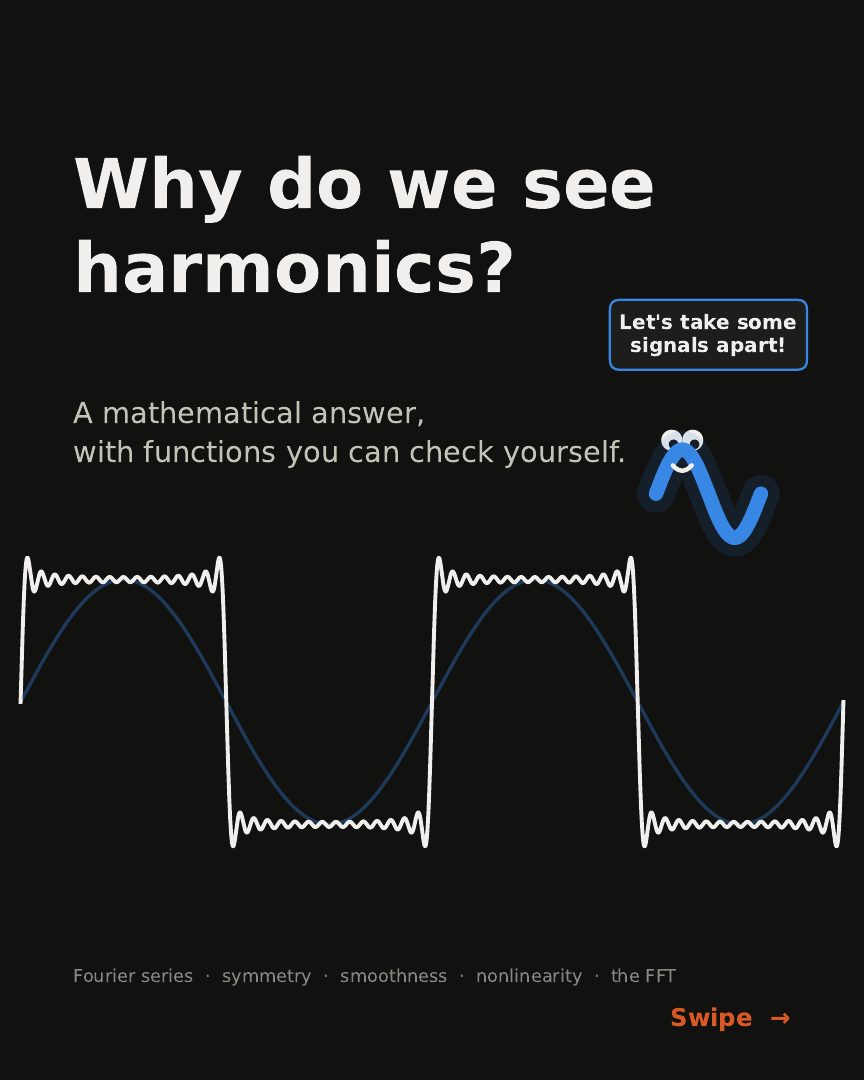
Why do we see harmonics?
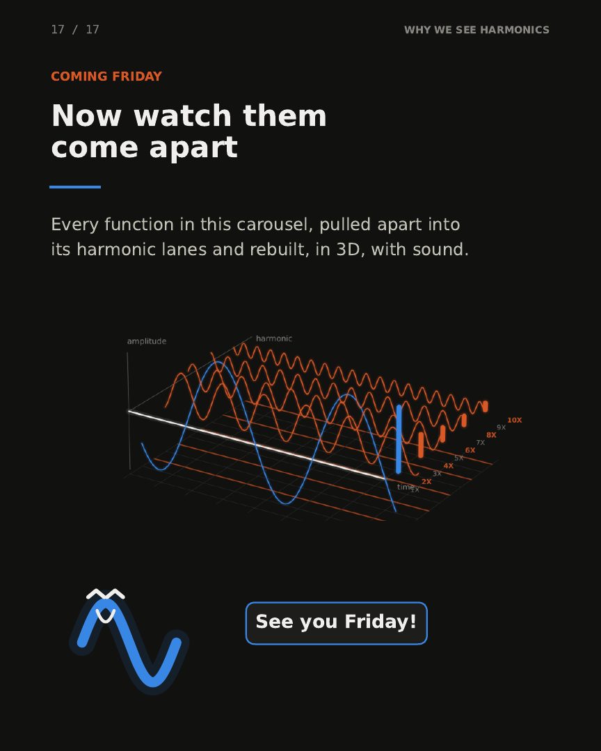
A mathematical answer, with functions you can check yourself. This is the full version of the LinkedIn carousel.
The carousel
Try it: build a signal from its harmonics
Pick a shape, then add harmonics one at a time. The solid line is the sum so far, the dashed line is the shape you are aiming for, and the spectrum shows each harmonic's amplitude (faded bars are the ones you haven't added yet).
The argument in seven steps
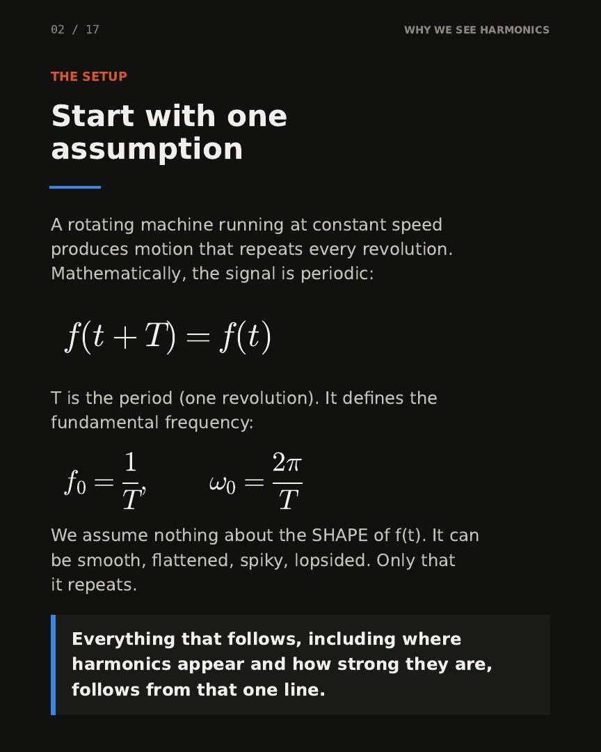
1. One assumption
A machine at constant speed produces motion that repeats every revolution. Mathematically the signal is periodic, with period \(T\) (one revolution):
Nothing is assumed about the shape: smooth, flattened, spiky or lopsided. Only that it repeats.
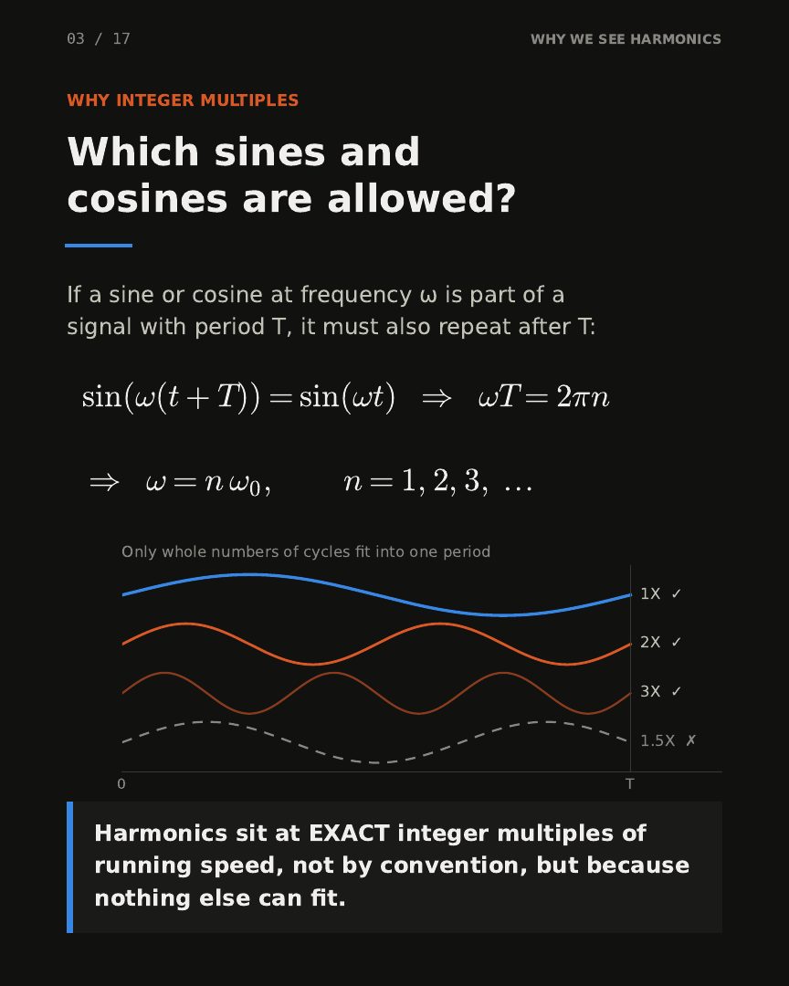
2. Only whole multiples fit
If a sine or cosine at frequency \(\omega\) is part of that signal, it has to repeat after \(T\) as well:
Harmonics sit at exact integer multiples of running speed, not by convention, but because nothing else fits.
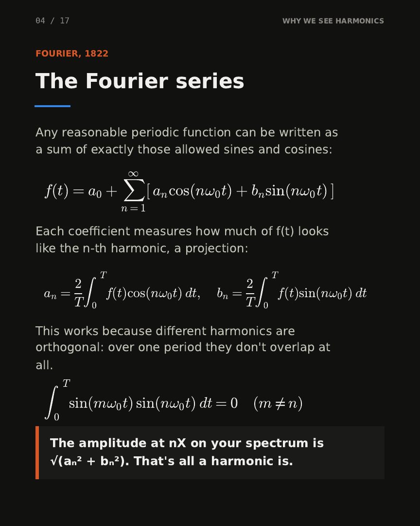
3. The Fourier series
Fourier (1822) showed that any reasonable periodic function is a sum of exactly those allowed sines and cosines:
Each coefficient measures how much the signal looks like that harmonic, a projection over one period:
The peak at \(n\)X on your spectrum is \(|c_n| = \sqrt{a_n^2 + b_n^2}\). That is all a harmonic is.
4. Worked examples
| Shape | Series | What you see |
|---|---|---|
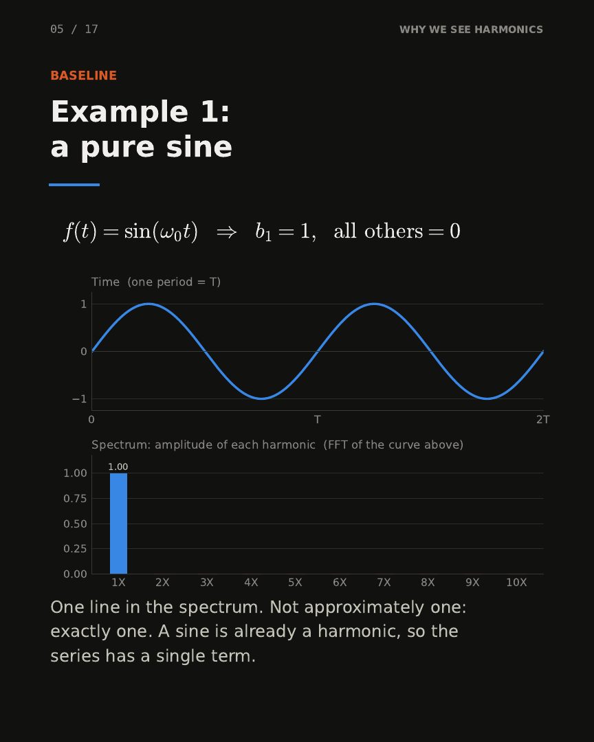
| Pure sine | \(\sin(\omega_0 t)\) | One peak at 1X |
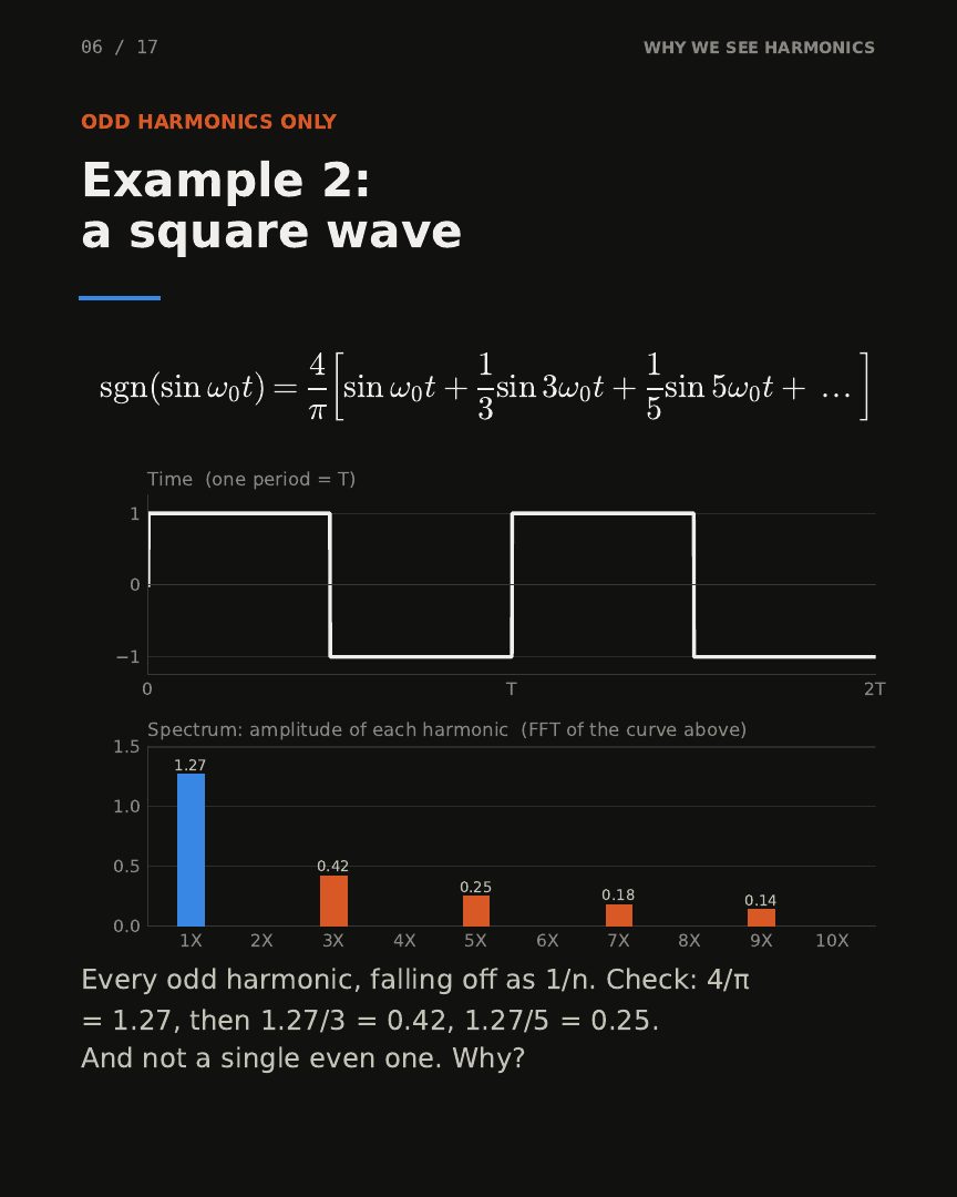
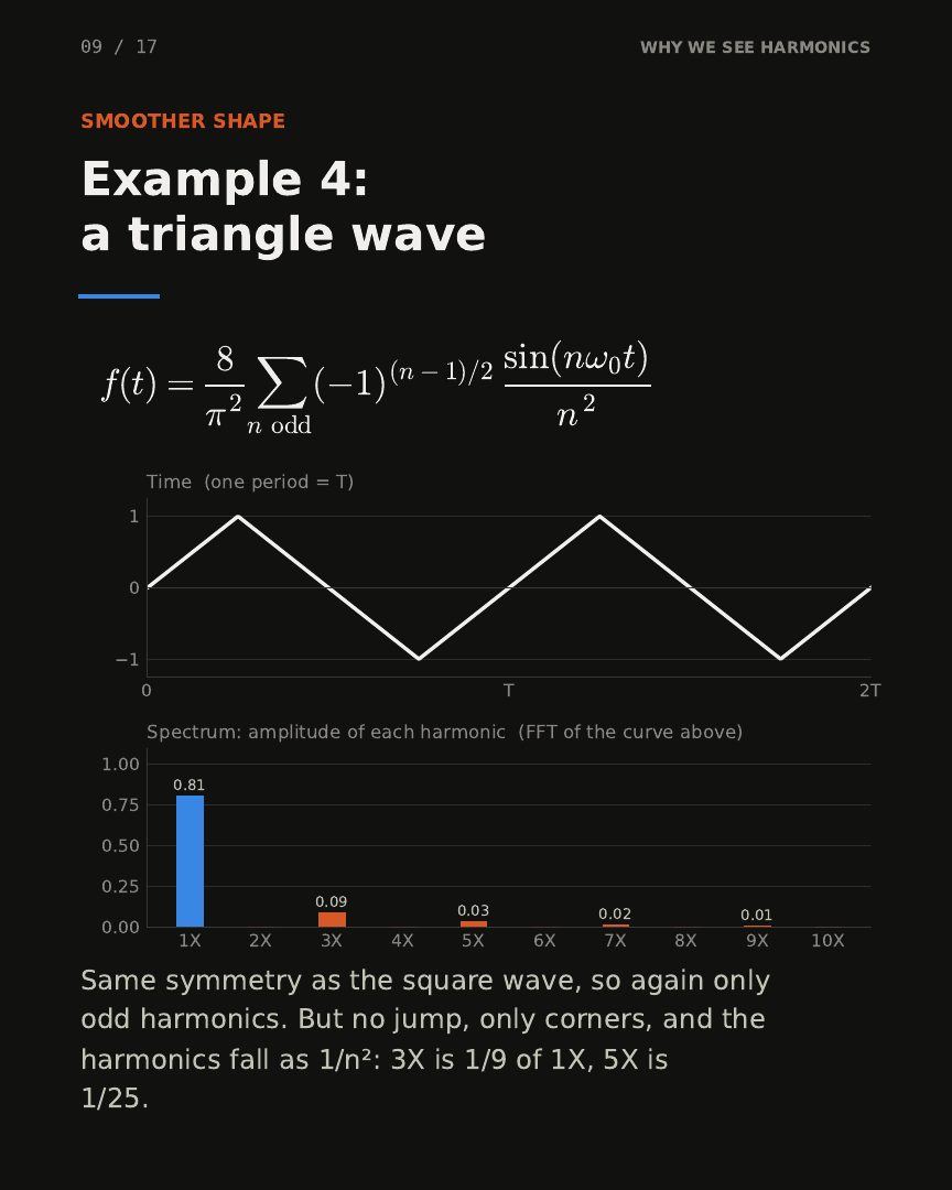
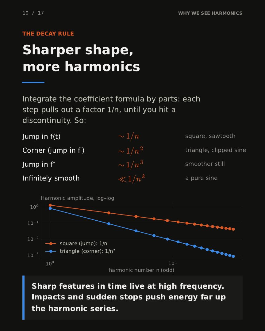
| Square | \(\frac{4}{\pi}\sum_{n\ \text{odd}}\frac{\sin(n\omega_0 t)}{n}\) | Odd only, 1.27, 0.42, 0.25, … (falls as \(1/n\)) |
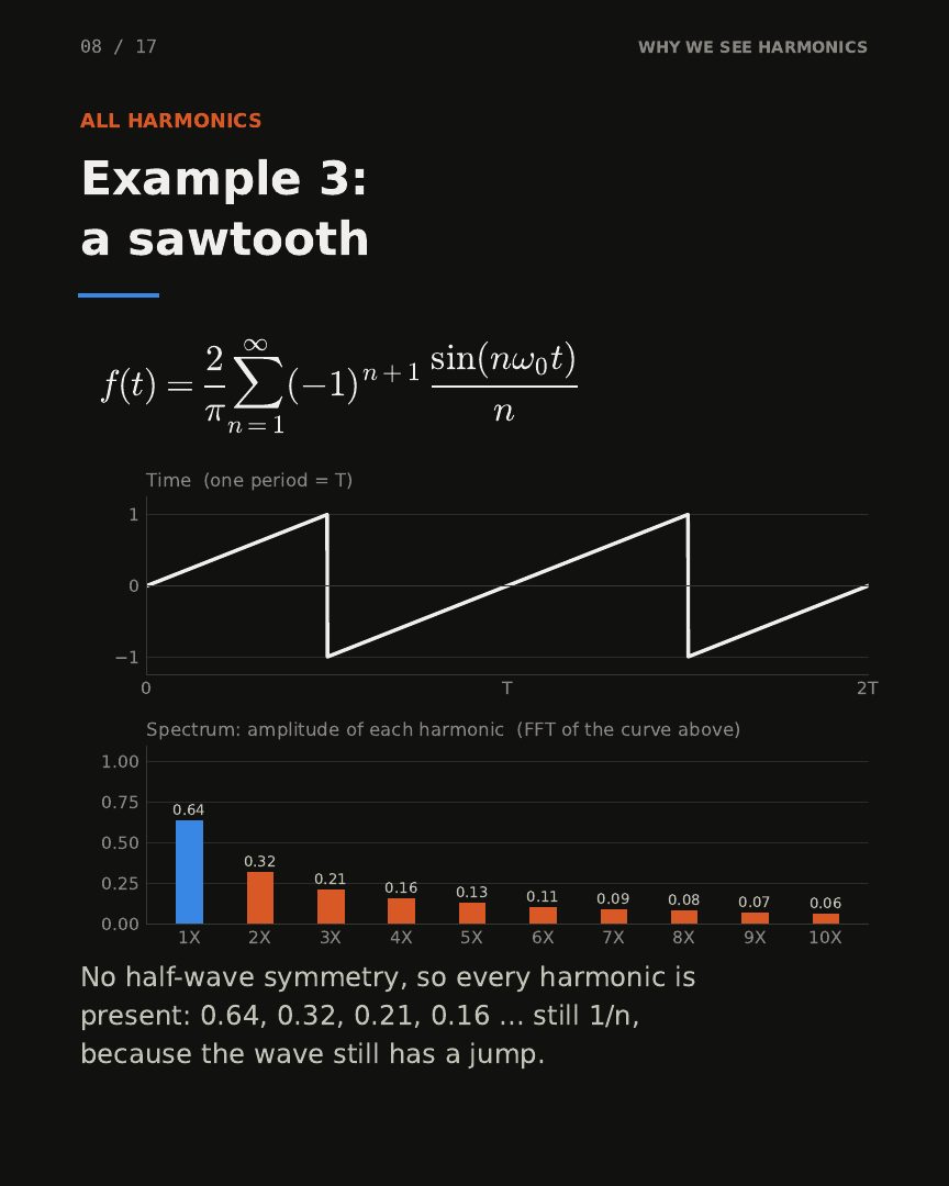
| Sawtooth | \(\frac{2}{\pi}\sum_{n}(-1)^{n+1}\frac{\sin(n\omega_0 t)}{n}\) | Every harmonic, 0.64, 0.32, 0.21, … (\(1/n\)) |
| Triangle | \(\frac{8}{\pi^2}\sum_{n\ \text{odd}}(-1)^{\frac{n-1}{2}}\frac{\sin(n\omega_0 t)}{n^2}\) | Odd only, falls as \(1/n^2\): 3X is 1/9 of 1X |
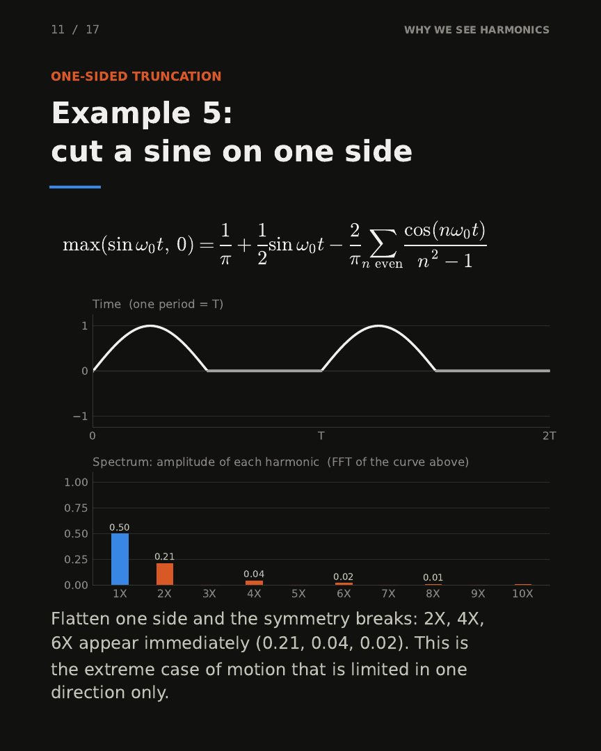
| Sine cut on one side | \(\frac{1}{\pi}+\frac{1}{2}\sin\omega_0 t-\frac{2}{\pi}\sum_{n\ \text{even}}\frac{\cos(n\omega_0 t)}{n^2-1}\) | 1X plus even harmonics, and a DC offset of \(1/\pi\) |
5. Symmetry decides odd vs even
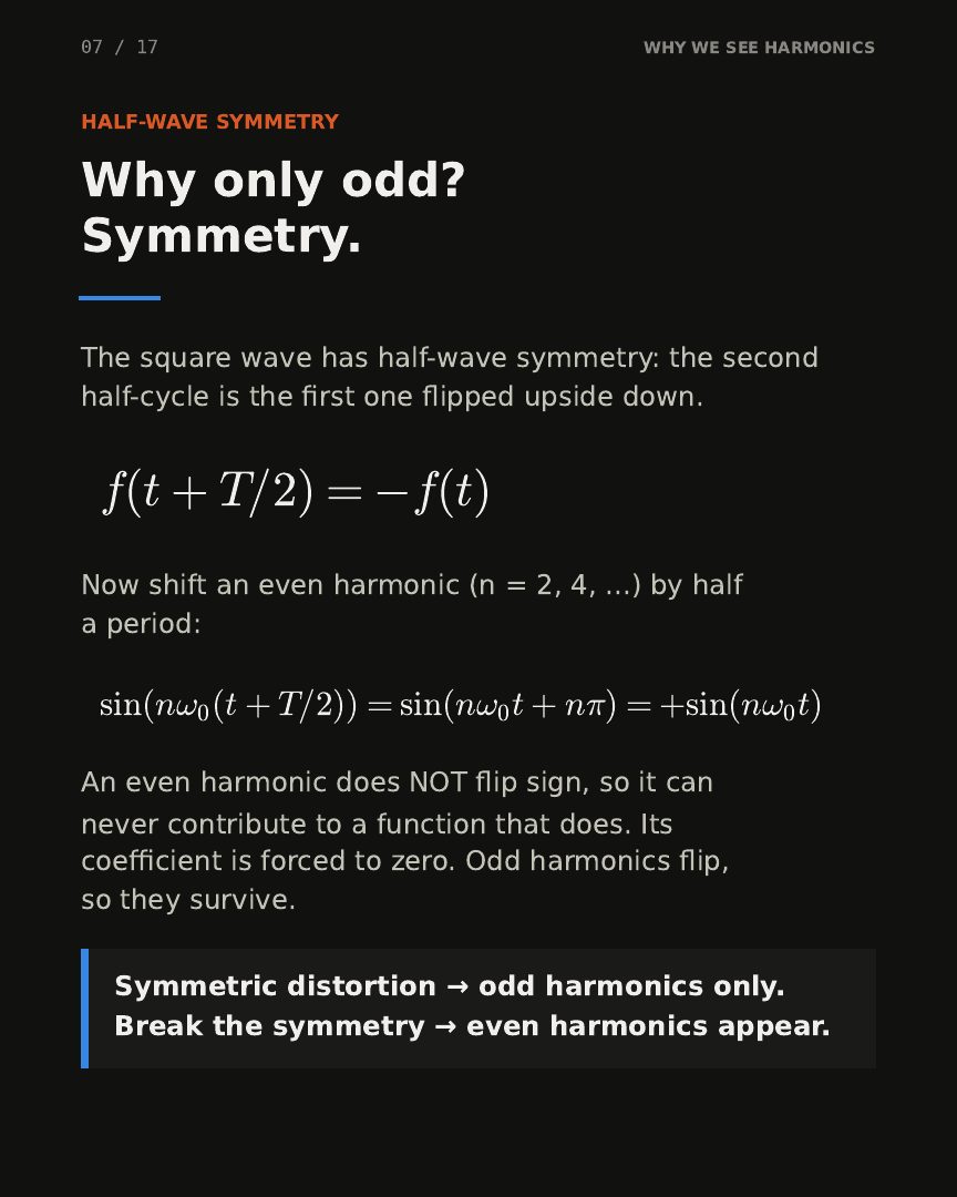
A square wave has half-wave symmetry: the second half-cycle is the first one flipped upside down, \(f(t+T/2) = -f(t)\). Shift an even harmonic by half a period and it lands on itself:
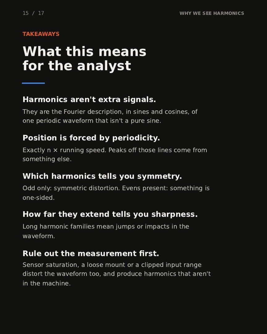
It doesn't flip, so it can't help build a shape that does: its coefficient is forced to zero. Odd harmonics flip, so they survive. Symmetric distortion gives odd harmonics only; break the symmetry and the evens appear.
6. Sharpness decides how far they extend
Integrate the coefficient formula by parts and each step pulls out a factor \(1/n\), until you hit a discontinuity. So a jump in the waveform gives harmonics that decay like \(1/n\), a corner gives \(1/n^2\), and smoother shapes decay faster still. Sharp features in time live at high frequency, which is why impacts push energy far up the harmonic series.
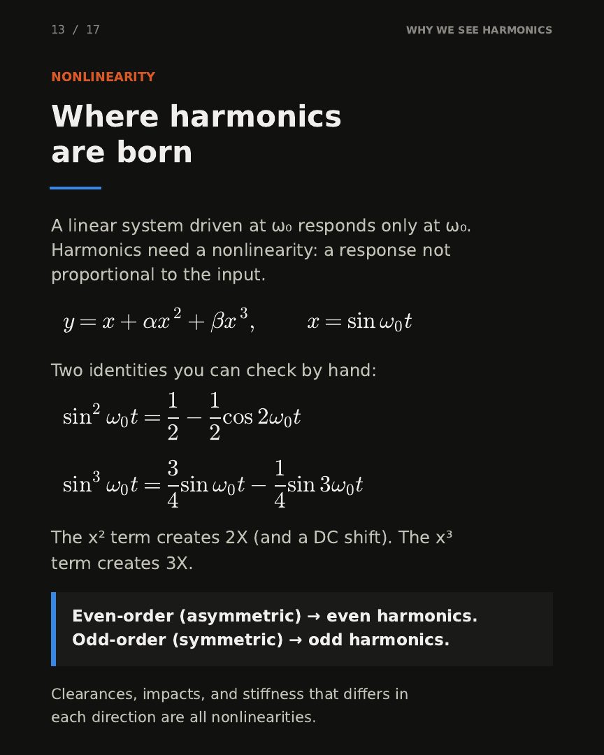
7. Where harmonics are born: nonlinearity
A linear system driven at \(\omega_0\) responds only at \(\omega_0\). Harmonics need a response that isn't proportional to the input. Two identities you can check by hand:
A squared (asymmetric) term creates 2X and a DC shift; a cubed (symmetric) term creates 3X. Clearances, impacts and stiffness that differs in each direction are all nonlinearities, which is why looseness and rubs show harmonic families.
Real signals
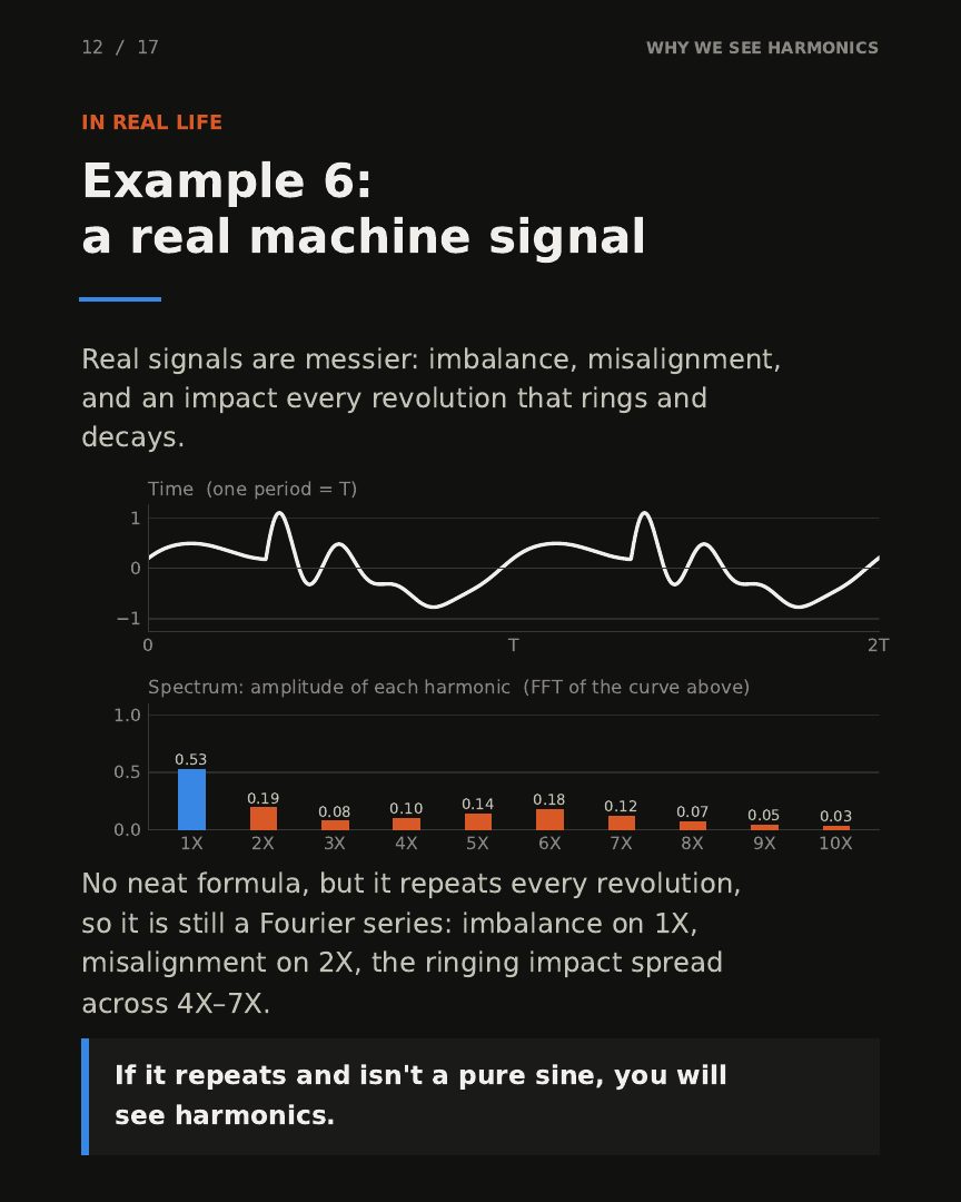
A real machine signal has no neat formula: some imbalance, some misalignment, an impact every revolution that rings and decays. But it still repeats, so it is still a Fourier series. Imbalance lands on 1X, misalignment on 2X, and the ringing impact spreads energy across 4X–7X. Select Real machine in the builder above to see it.
If something repeats and isn't a pure sine, you will see harmonics. They aren't extra signals: they're the shape of one repeating motion, written as sines and cosines.
A note on the FFT
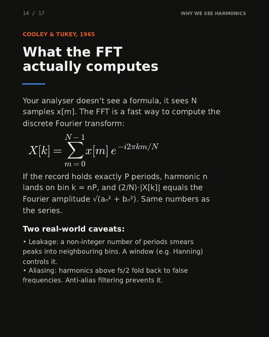
Your analyser doesn't see a formula, it sees samples. If the record holds a whole number of periods, harmonic \(n\) lands exactly on an FFT bin and \(\tfrac{2}{N}|X[k]|\) equals \(|c_n|\): the same numbers as the series. Two things break that in practice: leakage (a non-integer number of periods smears peaks into neighbouring bins; a window such as Hanning controls it) and aliasing (harmonics above half the sample rate fold back to false frequencies; anti-alias filtering prevents it). Before blaming the machine, rule out the measurement: a saturated sensor, a loose mount or a clipped input range also distort the waveform and create harmonics.
Check it yourself
The script below compares every series on this page with an FFT of the same function. The largest difference is about \(10^{-4}\), from sampling the jumps.
python verify_harmonics.py

function                                         n      FFT  formula
square     sgn(sin w0 t)                         1   1.2732   1.2732
                                                 3   0.4244   0.4244
                                                 5   0.2546   0.2546
...
Downloads
- why-we-see-harmonics.pdf · the 17-slide carousel
- verify_harmonics.py · checks every formula against an FFT (needs NumPy)
- harmonics_carousel.py · the script that builds the carousel (Matplotlib)
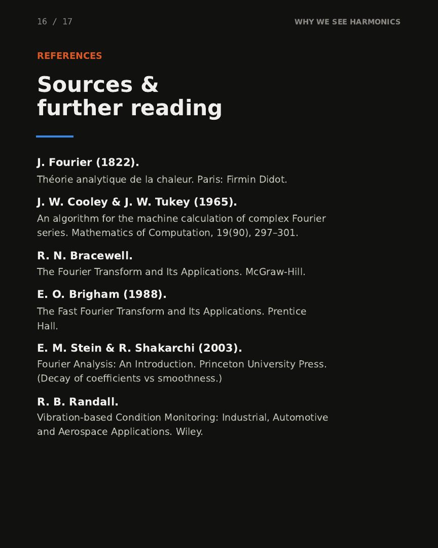
Sources and further reading
- J. Fourier (1822). Théorie analytique de la chaleur. Paris: Firmin Didot.
- J. W. Cooley & J. W. Tukey (1965). An algorithm for the machine calculation of complex Fourier series. Mathematics of Computation 19(90), 297–301.
- R. N. Bracewell. The Fourier Transform and Its Applications. McGraw-Hill.
- E. O. Brigham (1988). The Fast Fourier Transform and Its Applications. Prentice Hall.
- E. M. Stein & R. Shakarchi (2003). Fourier Analysis: An Introduction. Princeton University Press.Decay of coefficients vs smoothness.
- R. B. Randall. Vibration-based Condition Monitoring: Industrial, Automotive and Aerospace Applications. Wiley.